Measuring real-world benefits of breeding programs
Don’t guess: Add new data to statistical analysis
It is not hard to find out whether a breeding program actually increases farm production. If generations overlap in space and time at a farm, production data can be used to determine results without controlled benchmark studies.
Fig. 1 illustrates the kind of overlap the analysis requires. The large farm providing the data in Figure 1 stocked each successive generation over many months in many ponds, and usually had at least two generations growing simultaneously.
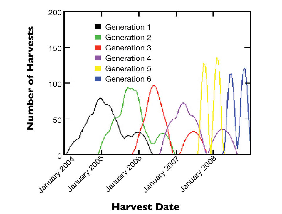
Given such overlapping data, it is possible to disentangle genetic and environmental effects on growth rate. The disentangling can be done statistically and does not require experimental growout in controlled environments. Nor does it require pedigree records, although each generation stocked in every pond must be identified.
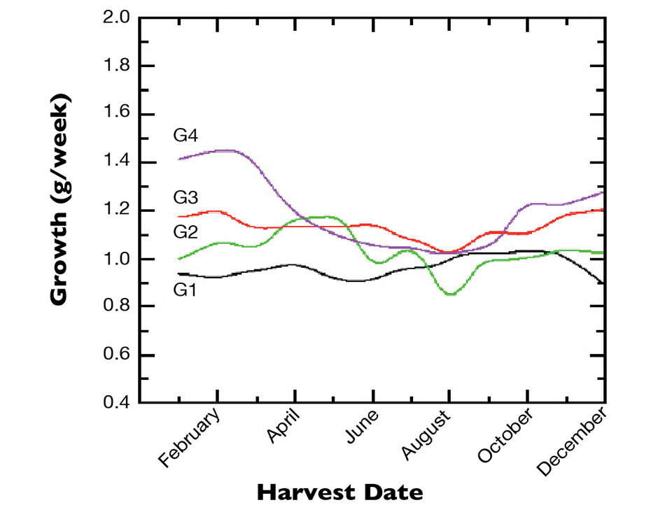
Fig. 2 illustrates a typical pattern of genetic gain at a large shrimp farm with many subfarms as it is expressed in different seasons of the year. There is a large spread of successive generations in some months but not others. The growth rate of shrimp harvested December through March appeared to increase almost 50 percent between generations 1 and 4. But the growth rate of shrimp harvested in the July-September period increased very little. The benefit from the breeding program was more or less zero for part of the year. So what was the real rate of genetic improvement?
Genetic improvement rate
There are two different answers, and both are correct. One says the genetic improvement varied 0-15 percent/generation depending on the season. This is neither more nor less than what one sees. However, when you know which generation was stocked in every pond, a more informative answer can be extracted: 11 percent/generation. This 11 percent is not an average.
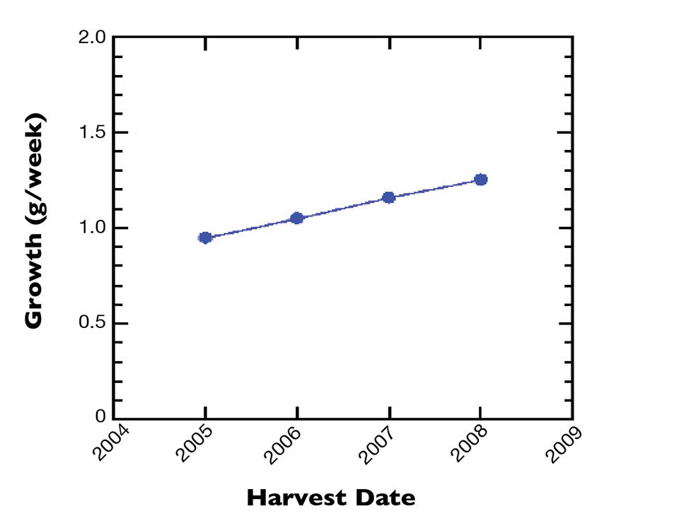
A simple average of raw data over all months and subfarms would be quite misleading for many reasons. A more accurate estimate requires statistical adjustment for “nuisance” environmental and management effects such as month, farm, region, pond bottom type, density and other variables. After adjustment, the growth rates shown in Fig. 2 increased steadily every generation (Fig. 3). The 11 percent/generation slope of the line in Fig. 3 goes up straight as an arrow.
It is a lamentable truth that controlled benchmark trials are worse than irrelevant if the spread between generations depends on the farm environment, as in Fig. 2. Whenever farm environments are less favorable or more variable than the benchmark – which is nearly always – the breeding program reports more rapid genetic gain than the farm.
Information transfer
Rather than benchmarking, it is more useful to put effort into a system of information transfer between the farm and breeding program that allows both parties to keep track of which generation grows in every pond. Genetic gain can then be estimated not by experimental field trials but by statistical analysis that disentangles the genetic and environmental effects in farm production data.
The real-world message in Figs. 2 and 3 is that the breeding program contributes more to farm production in good months than in bad. This observation can be generalized as the better the farm environment, the greater the benefit from genetic increases in growth rate.
In the absence of pedigree information, we cannot go beyond the simple observation that the spread of generations is environment-dependent. The root cause could be that different genes affect growth in good and bad environments or that genes with multiple effects are expressed differently in good and bad environments. Either way, disentangling genetic and environmental effects in farm data will estimate genetic gain correctly. We don’t need pedigree data to get that far.
Not only unfavorable seasonal environments can affect the expression of genetic gain. The author has seen similar reductions in the spread between generations when stocking density was so high it seriously reduced growth. Reduction in generational spread was also suspected, so far without definite proof, on a shrimp farm where feed quality was deliberately reduced as a cost-saving measure.
So there is no single rate of improvement per generation if the growout environment varies in time or space. It is entirely possible to see less genetic gain in farm ponds than in the breeding program and/or the selection environment and/or benchmark trials. Furthermore, some farm environments are intrinsically better than others, so two farms with identical genetics programs and starting broodstocks can have different rates of gain.
Other findings
The overlaps of generations, seasons, years, subfarms and ponds that allow us to disentangle genetic and environmental effects may allow us to discover other things, as well. Some of these findings may not be popular. For instance, the data may show that farm yield would fall every year if the breeding program were not continually improving the stock.
An example of this is seen in Fig. 4, where the observed growth rate at a large farm fluctuated around 1 gram per week between 2004 and 2008. The raw data are represented by the blue bars. After statistical adjustment for density, harvest month, etc., on-farm growth rate increased by 7.5 percent/year.
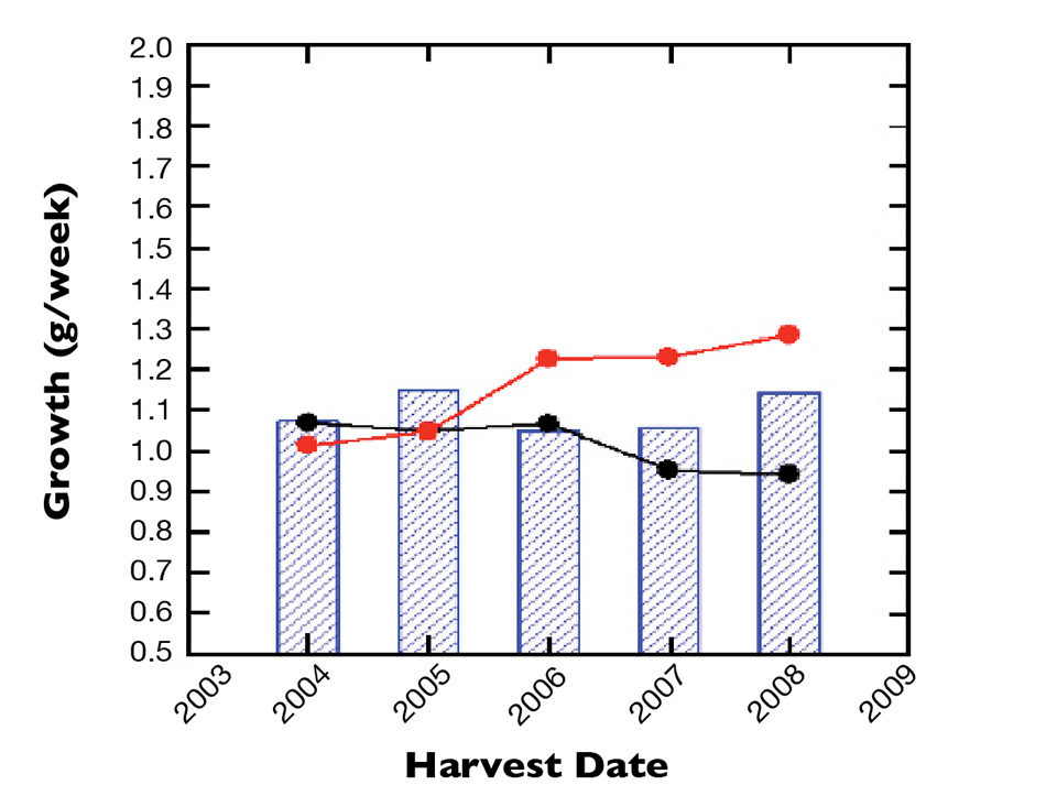
This doesn’t look too bad. Unfortunately, removing the contribution of all known environmental and management nuisance variables and genetic gain, the adjusted growth rate decreased by around 3 percent annually (black line). The benefit of the breeding program appeared to be cancelled by some negative change in the environment.
Statistical interaction
What was the cause of the unexplained, non-genetic downward trend in growth rate in Fig. 4? On this particular farm, we do not know. What we do know is that some important feature of the environment was missing from the factors and interaction terms in the statistical analysis.
What should be done if, upon disentangling generational and environmental effects, there seems to be a problem – a slow or fluctuating genetic gain as in Fig. 2, a deteriorating environment as in Fig. 4, or both?
A slow or fluctuating rate of genetic improvement does not necessarily require several specialized broodstock lines, such as summer and winter lines, or high- and low-density lines. Farm production data need to be associated with pedigree or equivalent data to make technical decisions about that. At the very least, the breeding program should focus selection on genes expressed favorably in the environment that most affect farm profit. If a bad environment or season is commercially important, then select accordingly.
If the grow-out environment is not only bad, but deteriorating, don’t guess why. Add new kinds of data to the statistical analysis. The factor that causes the problem is the one which, when included in the analysis, causes the disentangled, non-genetic annual trend (the black line in Fig. 4) to be horizontal or positive. When you have identified it in this way, you can take action to solve the problem on the farm.
(Editor’s Note: This article was originally published in the May/June 2009 print edition of the Global Aquaculture Advocate.)
Now that you've reached the end of the article ...
… please consider supporting GSA’s mission to advance responsible seafood practices through education, advocacy and third-party assurances. The Advocate aims to document the evolution of responsible seafood practices and share the expansive knowledge of our vast network of contributors.
By becoming a Global Seafood Alliance member, you’re ensuring that all of the pre-competitive work we do through member benefits, resources and events can continue. Individual membership costs just $50 a year.
Not a GSA member? Join us.
Author
-

Genetic Computation Ltd.
1-4630 Lochside Drive
Victoria, British Columbia
Canada V8Y2T1
Related Posts
Health & Welfare
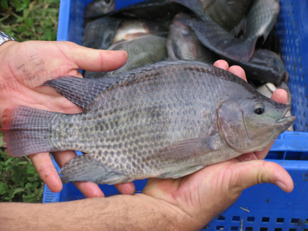
Applied commercial breeding program for Nile tilapia in Egypt
A major goal of selective breeding program for Nile tilapia (Oreochromis niloticus) in Egypt is to select for fillet color and fillet weight in response to consumer preferences.

Health & Welfare
‘Big picture’ connects shrimp disease, inbreeding
Disease problems on shrimp farms may be partly driven by an interaction between management practices that cause inbreeding in small hatcheries and the amplification by inbreeding of susceptibility to disease and environmental stresses.
Health & Welfare
A holistic management approach to EMS
Early Mortality Syndrome has devastated farmed shrimp in Asia and Latin America. With better understanding of the pathogen and the development and improvement of novel strategies, shrimp farmers are now able to better manage the disease.
Health & Welfare
10 paths to low productivity and profitability with tilapia in sub-Saharan Africa
Tilapia culture in sub-Saharan Africa suffers from low productivity and profitability. A comprehensive management approach is needed to address the root causes.